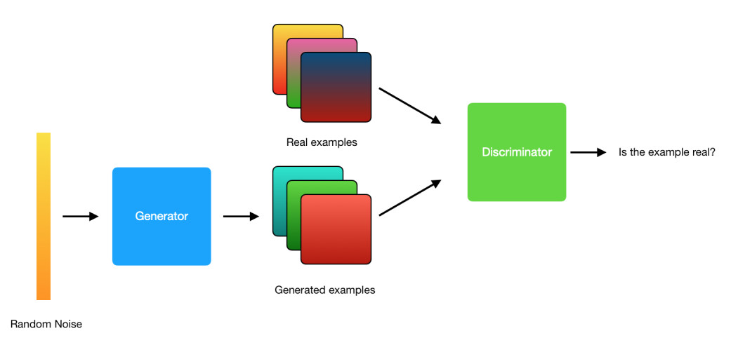
As the name suggests a Generative Adversarial Network is a network that creates or generates data, this data can be images, music, words, etc. In order to generate data, these networks learn to copy the distribution of the original data, we will see how we can build a GAN using a Deep Convolutional Generative Adversarial Network, this is a good architecture to start with.

We are going to use TensorFlow 2.0 due to the fact we can see the whole model creation and training process. For instance I suggest you to use Google Colab.

Generator and Discriminator models

A GAN is composed of two different neural networks, the Generator Network and the Discriminator Network, the generator is responsible for creating new examples of data, it takes as input a random noise (sometimes is called Z) and outputs data of the same format that the original data, for example if we have images of size 128x128x3 the generator will output an image of the same size. The discriminator will take the original data and the new created data (we usually call this fake data) and its job is to learn if the data is from the original distribution or if it is from the fake distribution.

We can say that the generator wants to create new data good enough to cheat the discriminator and make it think that the fake data is original data, at the same time the discriminator wants to learn when the data is original or fake.

You can check all the code of this post in this notebook.

The Generator

Now that we know the job of each network we will see how we can code these networks using TensorFlow:

def make_generator_model():

    model = tf.keras.Sequential()

    model.add(layers.Dense(8*8*1024, use_bias=False, input_shape=(100,)))

    model.add(layers.BatchNormalization())

    model.add(layers.LeakyReLU())



    model.add(layers.Reshape((8, 8, 1024)))

    assert model.output_shape == (None, 8, 8, 1024)



    model.add(layers.Conv2DTranspose(512, (5, 5), strides=(2, 2), padding='same', use_bias=False))

    assert model.output_shape == (None, 16, 16, 512)

    model.add(layers.BatchNormalization())

    model.add(layers.LeakyReLU())



    model.add(layers.Conv2DTranspose(256, (5, 5), strides=(2, 2), padding='same', use_bias=False))

    assert model.output_shape == (None, 32, 32, 256)

    model.add(layers.BatchNormalization())

    model.add(layers.LeakyReLU())



    model.add(layers.Conv2DTranspose(128, (5, 5), strides=(2, 2), padding='same', use_bias=False))

    assert model.output_shape == (None, 64, 64, 128)

    model.add(layers.BatchNormalization())

    model.add(layers.LeakyReLU())



    model.add(layers.Conv2DTranspose(64, (5, 5), strides=(2, 2), padding='same', use_bias=False))

    assert model.output_shape == (None, 128, 128, 64)

    model.add(layers.BatchNormalization())

    model.add(layers.LeakyReLU())



    model.add(layers.Conv2DTranspose(3, (5, 5), strides=(1, 1), padding='same', use_bias=False, activation='tanh'))

    assert model.output_shape == (None, 128, 128, 3)



    return model

As I previously mentioned the generator model takes as input a random noise called Z and outputs data of the same format that the original data, in this case an image of size 128x128x3, this model uses convolutional transpose layers since the model has to make the input bigger until it reaches the desire size of 128x128x3. We can notice that we use the tanh activation function due to the fact we want the output image to be in the range of [-1, 1]

Let's see how we can plot an image generated by this model:

generator = make_generator_model()



noise = tf.random.normal([1, 100])

generated_image = generator(noise, training=False)

Firt we create an instance of the model and use a random noise as input.

numpy_images = generated_image.numpy()

scaled_images = (((numpy_images - numpy_images.min()) * 255) / (numpy_images.max() - numpy_images.min())).astype(np.uint8)



plt.imshow(scaled_images[0])

Matplotlib needs the image to be in the range [0, 255], therefore, we scale the image before plotting.

Finally we obtain a new image:

The Discriminator

This model is easer to understand since it works like a normal network, it takes as input an image and outputs a prediction:

def make_discriminator_model():

    model = tf.keras.Sequential()

    model.add(layers.Conv2D(64, (5, 5), strides=(2, 2), padding='same',

                                     input_shape=[128, 128, 3]))



    assert model.output_shape == (None, 64, 64, 64)

    model.add(layers.LeakyReLU())

    model.add(layers.Dropout(0.3))



    model.add(layers.Conv2D(128, (5, 5), strides=(2, 2), padding='same'))

    assert model.output_shape == (None, 32, 32, 128)

    model.add(layers.LeakyReLU())

    model.add(layers.Dropout(0.3))



    model.add(layers.Conv2D(256, (5, 5), strides=(2, 2), padding='same'))

    assert model.output_shape == (None, 16, 16, 256)

    model.add(layers.LeakyReLU())

    model.add(layers.Dropout(0.3))



    model.add(layers.Conv2D(512, (5, 5), strides=(1, 1), padding='same'))

    assert model.output_shape == (None, 16, 16, 512)

    model.add(layers.LeakyReLU())

    model.add(layers.Dropout(0.3))



    model.add(layers.Conv2D(1024, (5, 5), strides=(2, 2), padding='same'))

    assert model.output_shape == (None, 8, 8, 1024)

    model.add(layers.LeakyReLU())

    model.add(layers.Dropout(0.3))



    model.add(layers.Flatten())

    model.add(layers.Dense(1, activation=None))



    return model

Then we can pass the generated image and see the prediction made by the discriminator:

discriminator = make_discriminator_model()

decision = discriminator(generated_image)

print(decision)

We want the discriminator to predict a number near to 1 if the input image is real and a number near to 0 if the input image is fake.

The dataset

We know that our generator outputs images of size 128x128x3 and the discriminator takes as input these generated images but we also need the real images that the generator will learn from, in this case we will use a dataset of famous people faces, we can download this dataset from Kaggle. Once we have the folder with the images we can create a generator with TensorFlow:

folder_name = 'img_align_celeba'

images_dir = os.listdir(folder_name)



all_image_paths = ilepaths = [os.path.join(folder_name, img_dir) for img_dir in images_dir]



buffer_size = len(images_dir)

batch_size = 128

train_steps = int(buffer_size / batch_size)

img_size = 128

In the code above we load all the paths from the images folder, we also indicate the final size of these images and the batch size.

def load_images(image_path):  

  image = tf.image.decode_jpeg(tf.io.read_file(image_path), channels=3)

  image = tf.image.convert_image_dtype(image, tf.float32)

  image = image / 127.5

  image = image - 1.

  image = tf.image.resize(image, [img_size, img_size])



  return image



dataset = tf.data.Dataset.from_tensor_slices(all_image_paths).shuffle(buffer_size)

dataset = dataset.map(load_images)

dataset = dataset.batch(batch_size)

Now with tf.data.Dataset.from_tensor_slices we create a generator that will load the images in batches.

The loss function

In order to train these networks we need a loss function, in fact we will use three loss functions.

cross_entropy = tf.keras.losses.BinaryCrossentropy(from_logits=True)

All the loss functions will use the binary cross entropy function since we are going to compare two outputs.

Discriminator loss function

def discriminator_loss(real_output, fake_output):

    real_loss = cross_entropy(tf.ones_like(real_output), real_output)

    fake_loss = cross_entropy(tf.zeros_like(fake_output), fake_output)

    total_loss = real_loss + fake_loss

    return total_loss

The discriminator's loss function takes the real images and the fake images created by the generator, in real_loss we want the discriminator to predict 1's whereas in fake_loss we want the discriminator to predict 0's, for instance we use tf.zeros_like and tf.ones_like to create a list of these numbers. Therefore in an ideally situation we would have:

real_loss = cross_entropy([1, 1, 1, 1, 1], [1, 1, 1, 1, 1])

and

fake_loss = cross_entropy([0, 0, 0, 0, 0], [0, 0, 0, 0, 0])

Finally we sum these two losses to obtain the total loss.

Generator loss function

In this loss we only take the predictions made by the discriminator, we want to cheat the discriminator, for instance we want these predictions to be 1's:

def generator_loss(fake_output):

    return cross_entropy(tf.ones_like(fake_output), fake_output)

Training

We need two optimizers since both networks have different parameters:

generator_optimizer = tf.keras.optimizers.Adam(1e-4)

discriminator_optimizer = tf.keras.optimizers.Adam(1e-4)

We will use the following hyperparameters:

epochs = 25

noise_dim = 100

num_examples_to_generate = 16



seed = tf.random.normal([num_examples_to_generate, noise_dim])

Now we create a function where we compute the loss function and update the parameters:

@tf.function

def train_step(images):

    noise = tf.random.normal([batch_size, noise_dim])



    with tf.GradientTape() as gen_tape, tf.GradientTape() as disc_tape:

      generated_images = generator(noise, training=True)



      real_output = discriminator(images, training=True)

      fake_output = discriminator(generated_images, training=True)



      gen_loss = generator_loss(fake_output)

      disc_loss = discriminator_loss(real_output, fake_output)



    gradients_of_generator = gen_tape.gradient(gen_loss, generator.trainable_variables)

    gradients_of_discriminator = disc_tape.gradient(disc_loss, discriminator.trainable_variables)



    generator_optimizer.apply_gradients(zip(gradients_of_generator, generator.trainable_variables))

    discriminator_optimizer.apply_gradients(zip(gradients_of_discriminator, discriminator.trainable_variables))

We can notice that the first step we take is to generate new images (generated_images) then the discriminator takes as input these generated images and the real images, we use the discriminator's predictions to compute the loss functions, finally we compute the gradients of each network (Backpropagation step) and the Gradient descent.

Now we can use this function multiple times to train both networks:

def train(dataset, epochs):

  for epoch in range(epochs):

    print(f"Starting epoch: {epoch + 1}/{epochs}")

    start = time.time()



    step = 0

    for image_batch in dataset:

      if step % 100 == 0:

        print(f"step: {step}/{train_steps}")



      step += 1 

      train_step(image_batch)



    checkpoint.save(file_prefix = checkpoint_prefix)



    print ('Time for epoch {} is {} sec'.format(epoch + 1, time.time()-start))