We know that Neural Networks have a black-box nature, this means that Neural Networks are hard to interpret. For instance we are not sure what are the decisions that the model makes or why the model makes this decisions. Class activation maps can help us to understand more our models, this technique works with Convolutional Neural Networks and show us know what regions of the image were relevant to make the prediction. The results can be pretty good as we will see.

You can see all the code of this tutorial in this notebook.

In this tutorial we are going to use tf.keras. However you can use plain Keras if you want. These two implementations are almost identical.

Network architecture

In order to obtain these activation maps we must add some layers at the end of our network. We will use the Mobile Net v2 architecture but you can use whatever you want.

First we have to get the last convolutional layer in our network, in Mobile Net v2 this is the antepenultimate layer:

def create_model():

  mobile_model = MobileNetV2(

       weights=None,

       input_shape=input_img_size,

       alpha=1,

       include_top=False)



  for layer in mobile_model.layers:

    layer.trainable = True



  # Last convolutional layer

  model = mobile_model.layers[-3].output

Now we have to add a Global Average Pooling layer after the last convolutional layer:

model = layers.GlobalAveragePooling2D()(model)

Finally we have to add a Dense layer, this layer have a softmax activation function. Even if we only have two classes we must use this activation function:

model = layers.Dense(2, activation="softmax", kernel_initializer='uniform')(model)



model = Model(inputs=mobile_model.input, outputs=model)



return model

Our complete model is:

def create_model():

  mobile_model = MobileNetV2(

       weights=None,

       input_shape=input_img_size,

       alpha=1,

       include_top=False)



  for layer in mobile_model.layers:

    layer.trainable = True



  model = mobile_model.layers[-3].output



  model = layers.GlobalAveragePooling2D()(model)



  model = layers.Dense(2, activation="softmax", kernel_initializer='uniform')(model)



  model = Model(inputs=mobile_model.input, outputs=model)



  return model

The Global Average Pooling layer takes the filters of the last convolutional layer and returns their average, the most important filters will have high signals.

The Dense layer will assign weights to the Global Average Pooling layer outputs for each class, this is the reason why we need a softmax activation function.

Dataset

We are going to use the MURA dataset, this dataset consist of images of bone X-rays, some of these images are abnormal, therefore we have two classes, abnormal and normal.

Since the original authors used class activation maps in this dataset it's a good example to show the potential of this technique.

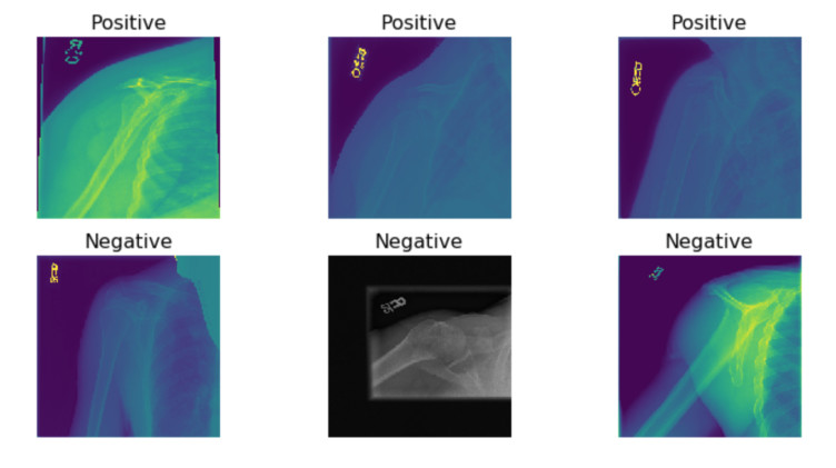
Some of the images.

Obtaining the activation maps

Once our network is trained we can take the activation maps from our last convolutional layer:

def get_activation_map(image_path, image_class_vector):        

        image_loaded = PIL.Image.open(image_path)

        image_loaded = image_loaded.resize((img_size, img_size))

        image_loaded = np.asarray(image_loaded)



        if len(image_loaded.shape) < 3:

          image_loaded = np.stack([image_loaded.copy()] * 3, axis=2)



        preprocessed_image = preprocess_input(image_loaded)

        preprocessed_image = np.expand_dims(preprocessed_image, axis=0)



        image_class = np.argmax(image_class_vector)



        class_weights = model.layers[-1].get_weights()[0]

        final_conv_layer = model.layers[-3]



        get_output = tf.keras.backend.function([model.layers[0].input], 

                                               [final_conv_layer.output, model.layers[-1].output])



        [conv_outputs, predictions] = get_output(preprocessed_image)

        conv_outputs = conv_outputs[0, :, :, :]



        cam = np.zeros(dtype=np.float32, shape=conv_outputs.shape[0:2])



        for index, weight in enumerate(class_weights[:, image_class]):

          cam += weight * conv_outputs[:, :, index]



        cam /= np.max(cam)

        cam = cv2.resize(cam, (img_size, img_size))

        heatmap = cv2.applyColorMap(np.uint8(255 * cam), cv2.COLORMAP_JET)

        heatmap[np.where(cam < 0.2)] = 0



        img = heatmap * 0.5 + image_loaded

        cv2.imwrite("heatmap.jpg", img)

This code looks long but it's easy:

First we have to load the image to be classified:

image_loaded = PIL.Image.open(image_path)

image_loaded = image_loaded.resize((img_size, img_size))

image_loaded = np.asarray(image_loaded)



# Convert to RGB

if len(image_loaded.shape) < 3:

  image_loaded = np.stack([image_loaded.copy()] * 3, axis=2)



preprocessed_image = preprocess_input(image_loaded)

preprocessed_image = np.expand_dims(preprocessed_image, axis=0)

Some of the images are black and white. Therefore we need to convert them to RGB.

image_class = np.argmax(image_class_vector)

We also have to obtain the class of the image.

class_weights = model.layers[-1].get_weights()[0]

final_conv_layer = model.layers[-3]



get_output = tf.keras.backend.function([model.layers[0].input], 

                                       [final_conv_layer.output, model.layers[-1].output])



[conv_outputs, predictions] = get_output(preprocessed_image)

conv_outputs = conv_outputs[0, :, :, :]



cam = np.zeros(dtype=np.float32, shape=conv_outputs.shape[0:2])

If you are using plain Keras you have to change tf.keras.backend.function for K.function

In the code above we are creating a new function called get_output to obtain the output of the last convolutional layer and the predictions of the network.

In the cam variable we are creating an empty tensor of the same shape than the conv_outputs variable, this new variable will have our class activation map:

for index, weight in enumerate(class_weights[:, image_class]):

  cam += weight * conv_outputs[:, :, index]

We have to move through each weight and multiply this weight by each filter from the conv_outputs variable, this will create our activation map.

print("predictions", predictions)



cam /= np.max(cam)

cam = cv2.resize(cam, (img_size, img_size))

heatmap = cv2.applyColorMap(np.uint8(255 * cam), cv2.COLORMAP_JET)

heatmap[np.where(cam < 0.2)] = 0



img = heatmap * 0.5 + image_loaded

cv2.imwrite("heatmap.jpg", img)

Finally we have to merge the original image and the class activation map. We end up with a result like the following one:

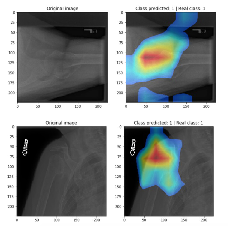
I have to mention that the neural network it's not too good, actually the accuracy in the training set is 80% and in the validation set is 76%. Despide the accuracy values, some activation maps are quite good and helpfully like the two in the last image. The MURA dataset contains some weird samples of bone X-rays like you can see in the notebook this makes the network harder to train. Data Augmentation helped to avoid overfitting since some images have zoom out perspectives we can apply this zoom out to all the images in the dataset.

More examples

We can use this technique in multiple datasets, for example the Retinal OCT dataset:

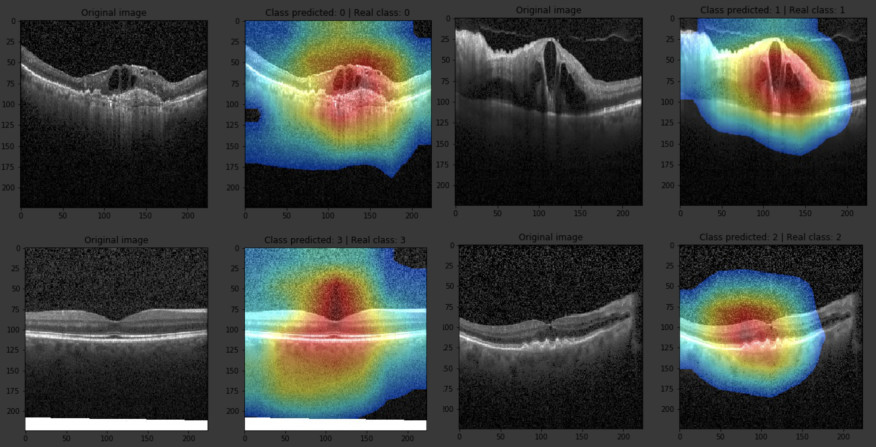
You can check the Jupyter Notebook here.

I have a post about how we can detect Alzheimer’s desease with deep learning where I use the activation maps as well, you can read it in this link.