In order to understand reinforcement learning, and before going deeper into novel approaches, let’s first understand a couple concepts:

Agent

An agent performs actions and interacts with the environment.

Environment

A defined space which allows interactions but no modifications.

State

The current position or situation of the Agent or parameters.

Action

A decision performed to change the current state.

Policy

The strategy used by the agent to take an action.

Policy function

Takes the current state as input and returns an action often P(a | s). It is the representation of the policy.

Policy model

The representation of the policy function as a machine learning model.

Markov chain

In the context of reinforcement learning, a Markov chain is a visual framework that represents the different interactions and states.

Value function

Estimates the base state or expected average return/reward from a chosen action. An action is expected to be better than the average.

Value model

Similar to the policy model, it is the representation of a value function as a machine learning model.

Reward function

Returns a positive or negative feedback to the taken action.

Value Based vs Policy Based

Policy based algorithms or models learn a mapping from states to actions (probabilities of the best next action), whereas Value based models estimates the expected return from a state, often a state-action pair, from which a policy or action is chosen as the next action.

Q-learning

Now, let’s observe how the previous concepts come together in one of the most popular classical reinforcement learning techniques, Q-learning, which proposal is the implementation of a Q-table to store the knowledge about the best possible actions and states:

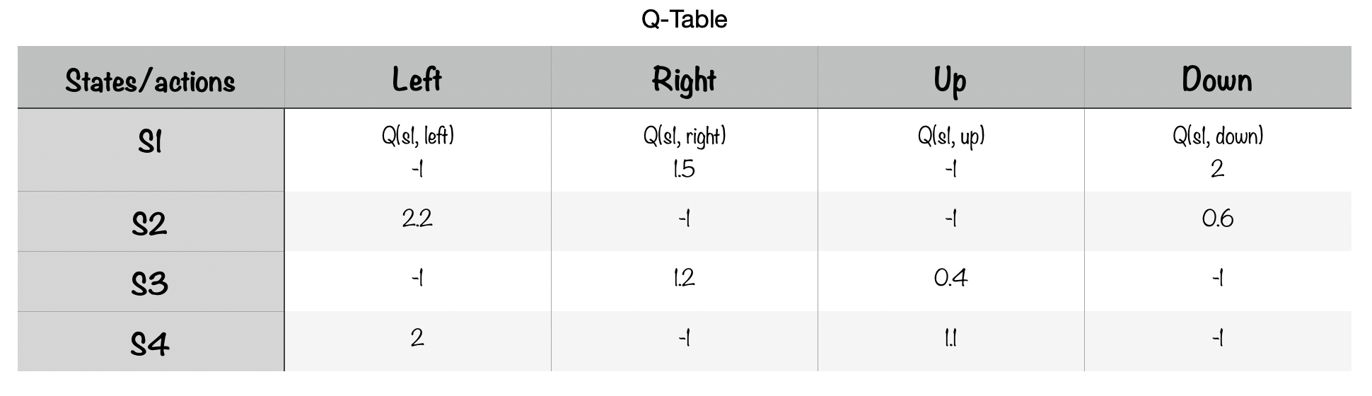
Rows represent the different states and columns the possible actions to take, the objective to optimize is the following equation:

Q(current state, action taken) = R(new state) +  y max Q(new state, best action)

Where y is a discount factor that reduces the importance of future actions

Defined as: Given the current state an action is taken, the result is the reward from the new state plus the reward from the best possible action taken in the new state.

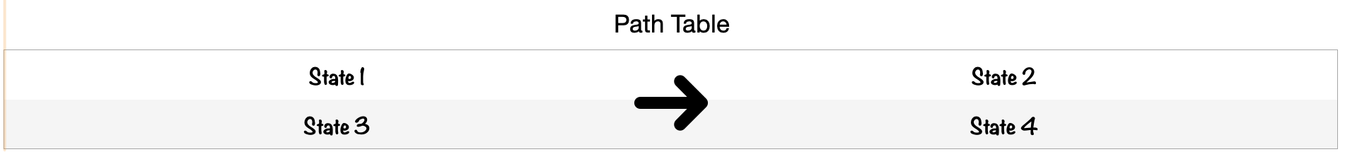
Once the algorithm is trained, one can rely on this table to perform actions. In the current Q-table state, if we want to take an action from state 2, the best option is to go left (2.2) (the worse would be go right or up). Looking at the path table, that means going to state S1 which best possible action is to go down (2), replacing in the equation:

Q(S2, left) = R(S1) + y max Q(S1, Down)
Q(S2, left) = 1.7 + (0.1) * 2 

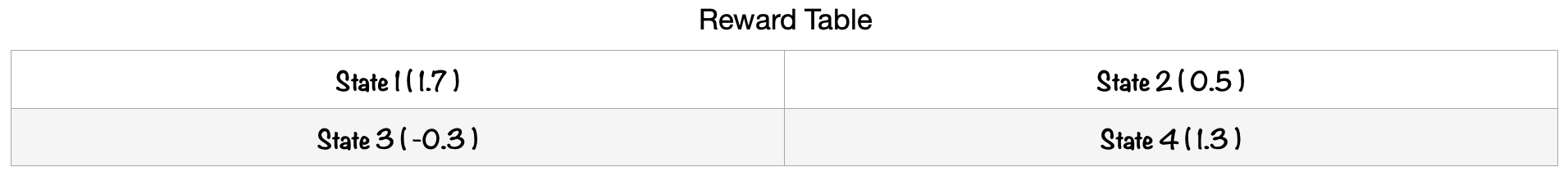
The reward table is employed to fill the first part of the equation “R(S1)”. For the second part, “Q(S1, Down)” the Q-table is used. In this way, Q(S2, left) returns 1.9 and our computed value was 2.2. The difference between both values is calculated, leading to the observed error used to update the Q-table:

Error = observed - expected (1.9 - 2.2)

Updates to:

Q(S2, left) = expected (Q(S2, left)) + alpha * error
Q(S2, left) = 2.2 + 0.2 (alpha) * - 0.3
Q(S2, left) = 2.14

Where alpha is the learning rate parameter.

To continue filling the table, this process is repeated until a stop criteria is met. As an additional note, you can follow two different approaches. The first is utilized to explore all the possible actions regardless of their rewards, and it is based on choosing just a random action (called exploration). The second is based on choosing the best path to obtain the best result (exploitation).

Learning can stop when the difference between the predicted and the reward values reach a threshold.

Even if the Q-table begins filled with zeros, if the reward function is correctly set up, each action probability will be updated correctly to inform the model the best action to take. To represent rewards, an additional table can be introduced, indicating what is the reward of going to some state.

Deep Q-networks

One massive drawback of Q-learning is its discrete area of action represented by the Q-table. Often, continuous outputs such as the movement of an object, cannot be correctly represented by the Q-table. Then, to address this issue Deep Q-networks introduce neural networks, replacing the Q-table and predicting the Q-values of all the possible actions by feeding just the current state. A Q-value is similar to the probability of a certain action but oriented to demonstrate how good the action is.

The well known gradient descent algorithm is then utilized to train the networks, requiring a loss function defined as the difference between the observed and expected outputs, similar to the Q-learning training but closer to a mean absolute error loss.

To replace the Q-table and maintain a stable training, an additional neural network called The target network is introduced. The later shares the same parameters (learning) and architecture as the Q-network but remains frozen for some steps.

The target network allows a more stable training by not forcing the Q-network to predict both the expected and observed values. Both networks work together in the following way:

1.- The Q-network predicts the expected value from where an action is chosen.

Expected_value = Q(current_state, current_action)

2.- The chosen or predicted action routes to the next state. The reward of this state is computed.

3.- The target network predicts the future Q-value from the next state.

MAX Q_target(next_state, next_action)

4.- Finally, the Q-network is updated by computing the loss.

Observed_value = R(next_state) + MAX Q_target(next_state, next_action)

Loss = (Observed - Expected)^2

At each step the predictions of the models: current_state, current_action, next_state, reward and, next_action are stored in a list called the experience replay memory.

In order to break the consecutive correlation between steps (state -> action -> new state -> new action) and improve stability, predictions from the former list are randomly sampled and used to train a batch.

After all these steps, the parameters of target network are replaced with the Q-network ones, and the process repeats.

Proximal Policy Optimization

While Q-learning tries to guide the agent following a policy, a policy algorithm suggests learning the policy itself. The later approach involves the outputs of neural networks, often a probability distribution after a softmax activation, to compose a loss function like:

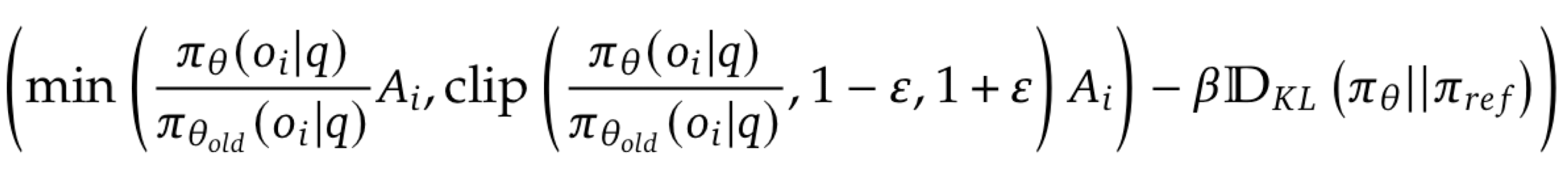
An advantage term A is computed from a value model to estimate the baseline (how good the average response/reward is) to beat by different rewards.

A vast number of regularization terms are introduced to guide a more stable training:

The first term quantifies how much the new model has changed relative to the old model (similar to Q-network, Target network), using the output probabilities of both models. Where the old model is an old version of the policy model. For several steps the old version of the policy model is frozen, while the new is updated. After this process ends, the old policy model is updated to have the same weights as the new version. This is required to obtain small update steps and prevent aggressive changes.

The second term includes the same outputs from both models, which are now clipped to be in a range between 1-e and 1+e to prevent variating vastly the knowledge of the model. This range creates a trust region ensuring small and controllable updates that improve stability.

Each term is then scaled by the advantage. Finally, the term that results in the most moderate change is chosen.

To further regularize training, the Kl-diverge is introduced as a third term. This diverge measures the difference between two distributions, in this case the policy model and an additional reference model. The later is often a model which knowledge wants to be kept and remains frozen during the most part of the training, only being replaced after a determinate number of training steps.

Group Relative Policy Optimization

A large disadvantage of the Proximal Policy Optimization algorithm is the integration of the additional value network, required to compute the baseline advantage. A novel approach, GRPO, addresses this issue by sampling a group of responses from the policy network and computing the average reward return (advantage) along this group. In this way, preventing the need of a value network.

A comparative of both approaches, where reward model does not need to be exactly a neural network but just a function designed to obtain a feedback according to the responses of the model. Both use basically the same loss function.

A group of questions is collected/created by annotators, for each question, G different responses {o1, o2, .., oN} (by variating the temperature parameter to achieve diversity) are sampled from old_model. Then, from G the expected advantage term A is calculated. The advantage reflects how good the average response is.

The advantage is computed by calculating the mean and standard deviation of the rewards of each response oi. Each response oi has its own advantage term (all tokens belonging to the same oi share the same advantage). Outputs oi should correctly answer the question to obtain a positive reward.

Inside the training step, new_model is feed the G different responses in the form: question + response (oi). The output is then used to compute the loss function as PI_0, and G responses as PI_old_0.

# where input_ids = each question + each response (oi) in G
outputs = new_model(input_ids)

log_probs = F.log_softmax(outputs.logits, dim=-1)

PI_0 = log_probs.gather(
  dim=-1,
  index=input_ids.unsqueeze(-1)
).squeeze(-1)

Log softmax is used to operate in the log space which is more stable with small values. (Addition instead of multiplication)

.gather returns the probability of the same tokens from input_ids, in other words:

• Given input_ids[i] = “The earth is …” generated by old_model.
• what is the probability assigned to each token [the, earth, is, …] by the new_model. Not the tokens with the highest probability, as commonly done.

A similar step is performed by the old_model to obtain the log probs, but also to sample the different responses. Here the tokens with the highest probability are chosen to form the response oi or PI_old_0.

Loss function is only computed over the response part tokens, not the question part tokens.

The rest of the training process is similar to PPO. Yet, way more efficient without the extra work of having a value network.

In the previous image the training flow can be observed. Split into the epochs loop, the batch loop and the update loop. Each part of the training can be understood such as the creation, training and update of old_model and reference_model. The sample of the G responses and questions. Inside the update loop, the former operations to calculate PI_0 are computed.